Some observations on the requirements for scale models to fly at scale speed.

In model aeroplane literature, more often than not, scale models are labelled as "difficult", the most common complaint being that of an airspeed too high for comfortable handling. A second consequence of the exaggerated velocity is that scale realism in the air tends to be poor. Curiously, the high speed seems to be widely regarded as an inherent property of scale models, and accepted without much further questioning. Slightly intrigued by this viewpoint, but more so by the offending mismatch in our perception of motion between full size and model, I began to look around for any aerodynamic laws to hold responsible for the trouble.

Scenario: If a certain full size aeroplane flies a distance equal to its own length in a certain amount of time, we would like the ideal scale model to fly a distance equal to its own length in exactly the same measure of time. True scale velocity, we may call it, and once we succeed in having a model perform this way, it will in level flight look quite like its full size counterpart seen further away.

The aim of this article is to
1) Show what it takes in terms of model properties to arrive at the desired velocity.
2) Show what kind of trouble we may expect to encounter in the process of scaling down.

Despite a somewhat concentrated search at the library on the topic of aeroplane model speed as compared to full size, all I ever managed to locate were vague hints in the direction of wing loading figures, whereas more specific hard-core information always seemed to evade any textbook or article I came across. Finally, curiosity made me sharpen my pencil and figure it out for myself. The results below do not pretend to be breathtaking news by any measure (some of them are indeed trivial), and no doubt they have all been presented elsewhere by numerous other persons many times in the past. Of the double-sided problem that I find it to be, namely one of weight and one of airfoil behaviour in the low Reynolds regime, the weight part is relatively simple and may easily be done with, while the second part is substantially more elusive, in worst cases uncontrollable to the point of overturning all efforts towards true scale velocity for the smallest of models.

Experimental Nieuport-17 built to 1/8 scale from white foam sheets of 5 mm thickness.
Wingspan 1 m, mass 135 gram (including 20 gram nose ballast).
Wing loading 0.6 kg/ sq meter. Glides at about 3 m/s.

---

Preliminaries:

Time is fixed. One second is one second, come what may.
Distance is 1-Dimensional, hence velocity (speed) is also 1D.
Area is 2D.
Volume is 3D, hence mass is also 3D.

Let r be the scale (reduction) factor.
For r = 12, the model is in scale 1/12

Scaling down, the distance shrinks to 1/r, the area shrinks to 1/r², the volume to 1/r³

When we say, for instance, that a model is in scale 1/12, we refer to the 1D properties (distances). From this fact follows that areas must be 1/ (12·12) and volumes must be 1/ (12·12·12).

---

Scale effects:

In order not to bore readers more than necessary, the outcome is presented first, the details and comments later for those who might want a closer look. In everything that follows, the subscript 1 stands for some property of the full size aeroplane, while subscript 2 is reserved for the model.

Rule 1    z₂ = z₁/r                  Wing loading, z, resulting from simple downscaling.
Rule 2    v₂ = v₁/sqrt(r)         Velocity, v, resulting from simple downscaling.
Rule 2a   v₂ = v₁/r                 True scale speed (velocity).
Rule 3    w₂ = w₁/r⁴               Mass, w, required to fly at true scale speed.
Rule 4    svz = z₁/r²               Scale velocity wing loading, svz, resulting from Rule 3

Conclusion 1 :   Concerning weight ( mass, to be correct ), there seems to be no principle which in itself prevents even the smallest of models from flying at scale velocity. Any limitation lies alone with our own abilities of very light construction. A precise number for the ideal mass is easily found.

Conclusion 2 :  Concerning airfoil performance, odd problems may considerably jeopardize very small scale model feasibility. The smaller the Reynolds number, the less the performance of any wing. More efficient non-scale wing profiles might be put to use, only still somewhere there will be an insurmountable barrier to the gain that can be attained this way, and so may Conclusion 2 in some cases trip Conclusion 1.

---

Rule 1

A property, often referred to when comparing aircraft, is the wing loading, z, i.e. total mass divided by wing area. If we scale down, the wing area diminishes by the square, whereas the volume, and hence mass, diminishes by the cube, that is, the mass shrinks faster than the area, which in turn means that the model always will have less wing loading than the full size plane. This principle of "lost" wing loading is also known - at least in the model aeroplane folklore - as the "square-cube" law. Quite clearly it will only be valid on the condition that the materials used for the model are of roughly the same density as those for the full size machine, and that the two structures are fairly similar.

Let w₁ and w₂ be the masses of the prototype and model respectively, and let S₁ and S₂ be the areas of the wing surfaces:
w₂ = w₁/r³       ( model mass, by simple downscaling )
S₂= S₁/r²        ( model wing area, by simple downscaling )
z₁ = w₁/S₁        ( full size wing loading )
z₂ = w₂/S₂ = (w₁/r³)·(r²/S₁) = w₁/ (r·S₁) = z₁/r
Wing loading for model ( by simple downscaling ) = full size wing loading / r

---

Rule 2

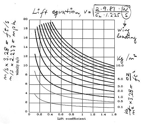
Of special interest for aeroplanes is the Lift Equation:    L = C_L·q·S
L = w·g = Newton ( N )
w = aeroplane total mass ( kg )
g = acceleration due to gravity = 9.81 m/s²      ( 32.2 ft/s² )
C_L = Lift Coefficient ( a dimensionless value to indicate the lift capacity of a certain shape )
q = d/2·v²
d = density of air = 1.225 kg/m³       ( 0.0765 lb/ft³ or, to be correct, 0.002377 slugs/ft³ )
v = velocity ( m/s )
S = surface area of wing ( m² )
S = c·b
c = mean wing chord ( m )
b = wingspan ( m )
The lift equation in full: w·g = C_L·d/2·v²·S
or, upon rearrangement: 2·w·g = C_L·d·v²·S
Rearranging for velocity squared: v² = 2·w·g / ( C_L·d·S)
Comparing model velocity to full size velocity:
v₂²/v₁² = (2·w₂·g·C_L·d·S₁) / (C_L·d·S₂·2·w₁·g) = (w₂·S₁) / (S₂·w₁) = z₂/z₁
Substituting z₂ by Rule 1 leads to:
v₂²/v₁² = z₁/(r·z₁) = 1/r
v₂² = v₁²/r
v₂ = v₁/sqrt(r)
Velocity for model ( by simple downscaling ) = full size velocity / squareroot of (r)

Of likely interest may also be to compare the original velocity, v₂, with the resultant velocity, v₃, in case just the model mass ( and hence wing loading ) is changed:
v₃ = v₂·sqrt(w₃/w₂)       or the equivalent:      v₃ = v₂·sqrt(z₃/z₂)

Ross says that for a small duration model ( e.g. Peanut scale, 13" wingspan ( 33 cm )), the best wing loading should be about 0.33 gram/in², and for a medium size plane ( about 30" ( 76 cm )), it should be somewhere around 0.5 gram/in². Converting these two figures to more familiar units:
Small: 0.33 gram/in²     = 0.50 kg/m²    (1.64 oz/ft² )
Medium: 0.50 gram/in² = 0.78 kg/m²     (2.56 oz/ft²)

These values, to be sure, are for duration models. From other sources I have found that R/C people are not particularly unhappy about quite large wing loadings, as long as they do not exceed 20 oz/ft² = 6.1 kg/m² (a crude average extract from several News group posts). So our Spitfire of 11 kg/m² apparently has a severe weight problem for rubber duration and R/C alike, besides the fact that it's totally out of range of true scale speed. Now, the 1.74 kg is a worst case example, and we would no doubt have little difficulty in building the model a lot lighter than that, only we still don't know just exactly how light it needs to be. What I will show you in a moment, is that we can actually develop a simple rule to determine the mass of the model so that it should fly at scale velocity, everything else being equal (which may not quite be the case). I shall give you the details shortly, but for now I can reveal that should our model be able to fly at 4.8 m/s, it would require that the mass be 0.145 kg, dramatically different from the 1.74 kg, and, as it were, exactly 1/12 of 1.74. The resultant wing loading would be 0.145/0.156 = 0.93 kg/m². Now take a second look at the value Ross gives for medium sized models. We are quite close.

---

Rule 3

Rearranging the lift equation for mass: w = C_L·d·v²·S / (2·g)
Under the somewhat bold assumption that C_L remains constant for the full size aeroplane and the model alike, we may write:
w₁ = C_L·d·v₁²·S₁ / (2·g)        ( mass of full size )
w₂ = C_L·d·v₂²·S₂ / (2·g)        ( model mass )
Comparing the two:
w₂/w₁ = (C_L·d·v₂²·S₂·2·g) / (2·g·C_L·d·v₁²·S₁) = (v₂²·S₂) / (v₁²·S₁)
v₂ = v₁/r       ( true scale velocity )
S₂ = S₁/r²       ( simple downscaling )
Inserting these expressions for v₂ and S₂ we get:
w₂/w₁ = (v₁/r)²·(S₁/r²) / (v₁²·S₁) = 1/r⁴
w₂ = w₁/r⁴
Model mass required to fly at true scale speed = full size mass / r⁴

This remarkably simple relation is the kind of information I originally went out to hunt.

Table of scale effect, resulting from Rule 3. Original mass = 3000 kg, original vel. = 58 m/s
Scale   Mass (gram)     Wing loading (kg/m²)     Scale speed (m/s)     Re (description below)
  1/4    11719                         8.33                                 14.5                            555000
  1/6      2315                         3.70                                   9.7                            247000
  1/8        732                         2.08                                   7.3                            139000
1/10        300                         1.33                                   5.8                              89000
1/12        145                         0.93                                   4.8                              62000
1/16          46                         0.52                                   3.6                              35000
1/24            9                         0.23                                   2.4                              15000
1/32            3                         0.13                                   1.8                                8700
1/48            0.6                      0.058                                 1.2                                3800
1/64            0.2                      0.033                                 0.9                                2100
1/72            0.1                      0.026                                 0.8                                1700

With regards to mass alone it appears that in principle there is no problem with scaling down and remain flying at scale speed. The finest successful example I have heard of so far (Walter Scholl, E-zone sep. 1997) is a Blériot XI, 1/10 scale model of 115 gram mass, electric engine and micro R/C included, and flying at scale speed 2 m/s. The wing loading is 0.46 kg/m², even less than Ross' smallest figure.
The practical construction of such extremely lightweight devices as required in the small scale regime may however not always come easy. Rule 3 is a serious enough constraint for small models. As to our 1/12 scale Spitfire above, we could easily find ourselves in a situation where we do not have sufficiently delicate components at hand to get away with anything more than a crude free-flight version.

Alarmingly primitive Bf 109 F prototype in mixed foam/balsa, built to 1/12 scale.
Although the artistic appearance of this my first foam job ever is nothing to be proud of, the aerodynamic properties are not bad at all. Wingspan 83 cm, Clark Y-ish airfoil.
Total mass 128 gram (including 34 gram nose ballast).
Glides at 4.5 m/s. Rate of descent is about 0.75 m/s.

Rule 3 may be expanded to include lift coefficients for full size and model, in cases where those values are known or can be guesstimated.
w₂ = (w₁/r⁴)·(C_L2/C_L1)

---

Rule 4

w₂ = w₁/r⁴    ( using Rule 3 )
S₂ = S₁/r²         ( by simple downscaling )
z₂ = w₂/S₂ = (w₁/r⁴)·(r²/S₁) = w₁/ (S₁·r²) = z₁/r²
Scale velocity wing loading = full size wing loading / r²  

One particularly attractive side effect of slow flying lightweight'ers is the low impact energy in collisions, making them extremely robust against major damage during encounters with trees and lampposts - not to forget that also they won't easily kill people.

---

Reynolds number ( Re ).

A quite different matter which has to be faced in the process of scaling down, is the aerodynamic behaviour of wing profiles (airfoils) operated at small dimensions and/or velocities, as would be required for small models.
To begin with the Reynolds number:
Viscosity, µ, may be expressed in Pascal·second,  Pa·s = (N/m²)·s = kg/(m·s)
µ (air) = 1.8 ·10^-5 Pa·s      [ For comparison, µ (water) = 1.0 ·10^-3 Pa·s; 55 times more viscous ]

Reynolds number (Re) = c·v·d/µ          
( c, v and d as defined earlier in details of Rule 2;   d/µ has the dimension second/m² )

With c in meter, and v in meter/second, Re = approximately 68000 · c · v
With c in feet, and v in feet/second, Re will be approx. 6410 · c · v

Full size aeroplanes have Re in the million class, whereas indoor models may come as low as 10000 (microfilm). Tables or plots of lift and drag coefficients as a function of angle of attack (AoA, or alpha) and different Reynolds numbers are valuable when comparing airfoils, as well as an indication of which dimensions and/or velocities better to be avoided for a specific wing profile. Data to this effect are most often obtained from wind tunnel tests, but also theoretical tools are capable of calculating fair predictions, as long as we make sure to stay above Re 100000. One such tool by Martin Hepperle is given in a link at the end of this web page. The book by Martin Simons, also listed below, devotes several chapters to the presentation and discussion of airfoil and wind tunnel data.

On eyeballing a number of wind tunnel plots, a coarse rule-of-thumb, which constitutes the advertised "barrier" in Conclusion 2, may be formed: Not many profiles can be pushed to a lift coefficient any higher than 1.5, a figure reached at an AoA of roughly 10°, dangerously close to the stall, and at the inconvenient expense of much increased air resistance. High-lift devices, flaps and slats, may boost the maximum lift coefficient to even twice that value, but once again with a price to be paid. For regular profiles at more modest AoA's and economical lift/drag ratios, the lift coefficients generally stay below 1.0
In the notes to Rule 3 it was mentioned in passing that lift coefficients for the full size plane and the model might not be quite the same value. Although it was a prerequisite for developing Rule 3, and may well be close enough to the truth for large models like 1/4 or 1/6 scale, it's not likely to be an equally safe assumption for smaller models, say 1/10 and less. The problem here is the almost total absence of linearity between the lifting capacity of two airfoils of equal proportions but different size. One cannot safely assume, without wind tunnel evidence or practical field experiments, that a downscaled version of some specific wing profile will have any relationship with the full size version in terms of efficiency; in fact an extensive amount of published data strongly indicates that the smaller of the two will show a markedly inferior performance, and that the trouble usually aggravates as we move towards the very low Reynolds regime. What happens here is that inertial forces to some extent loose their grip in a struggle against viscous forces. Let me give you a taste of what's to be expected, by a few examples, which, with the exception of EJ 85, are all drawn from Simons, more or less at random:

Reynolds numbers are by the thousands. In all cases the Angle of Attack is 3°

N60                                      NACA 4412                        Göttingen 801
 Re    cl    cd   cl/cd               Re      cl    cd   cl/cd            Re    cl    cd   cl/cd
168  .94  .021  44.8              3000  .75  .005 150.0           170  .88  .019  46.3
126  .93  .023  40.4                250  .70  .018   38.9           100  .88  .025  35.2
105  .90  .026  34.6                  75  .70  .030   23.3         +  75  .83  .035  23.7
  84  .87  .029  30.0                  60  .50  .048   10.4         +  75  .65  .050  13.0
  63  .50  .050  10.0                  45  .38  .054     7.0             63  .55  .060    9.2
  42  .44  .088    5.0                  30  .31  .060     5.2             42  .47  .066    7.1
  21  .42  .094    4.5                  20  .27  .068     4.0             21  .40  .066    6.1

Göttingen 417b                     HK 8556 [T]                        EJ 85
 Re    cl     cd    cl/cd              Re    cl    cd   cl/cd               Re    cl    cd   cl/cd
189 1.16  .028  41.4               120  .71  .027  26.3               83  .95  .025  38.0
  84   .86  .073  11.8                 60  .71  .030  23.7               60  .95  .038  25.0
  63   .65  .083    7.8                 30  .71  .068  10.4               40  .93  .060  15.5
  42   .59  .096    6.1                 20  .65  .085    7.6               20  .70  .046  15.2
  21   .76    ?        -
  14   .90    ?        -

A few notes:

Göttingen 801: Suspicious behaviour is seen around Re 75000 ( marked with + ), as part of a so-called hysteresis loop, with the effect that in a certain Re range, and specific AoA, the profile gives a better performance in going from higher to lower speed than in going from lower to higher. This unpleasant behaviour is shown by many profiles, including N60 and Gö 417b (at higher AoA than 3°), whereas this is not the case with NACA 4412, HK 8556 [T] and EJ 85. See Simons for details if you are interested.

Göttingen 417b, curved plate: Surprises in cl at Re 21000 and 14000, although most likely accompanied by large increases in profile drag (outside the limits of recording).

HK 8556 [T] Turbulator, and EJ 85: These profiles seem to offer the best alternatives at low velocities and/or dimensions. EJ 85 is a Jedelsky profile.

As seen in the previous few tables, it's evident that the highest lift coefficients coincide with the highest Reynolds numbers, and also that above a certain Re the gain in lift capacity with a further increase in Re is extremely limited, if any at all. In the low end of the Re scale, for most profiles the lift coefficients are more widely scattered with changes in Re. Drag coefficients, cd, move in the opposite direction of cl with changing Re number. Apart from that, any broad generalisation is difficult to make because of exceptions and surprises, thus rendering predictions a little hazy. Within a confined Reynolds region, e.g. around 60000, any change/improvement in performance seems to be possible only by exchanging the profile - if a suitable one is to be found. For real flying devices, matters are slightly more complicated, as most often we need to know the amount of power required for flight and/or the distance covered in a glide from a certain height. To this end various other drag components must be added to the profile drag and compared with the lift coefficients, in order to make a realistic estimate of the rate of descent and hence the usefulness of some particular wing in connection with the rest of the aeroplane. All this, however, is so much better described in textbooks like the ones by Simons and Stinton.

At present, it is believed that for very small models, the best job will be done by a thin, highly cambered wing profile, even such seemingly simple ones as the broken plate variation of a Jedelsky profile (see Don Ross). This again indicates that perfect scale appearance - for all but pre 1920 aeroplanes - may have to be sacrificed to some extent. In Aeromodeller, sep / oct 1997, vol 62, No 742 and 743, two articles "Foam at last!" by David Deadman, describe the construction of lightweight and extraordinarily realistic peanut scale models. I have been informed by the author that one of his planes, a Lavochkin La-7, scale approx 1/30 and mass 13 gram, flies at about 4.8 m/s, corresponding to 80 % of scale maximum speed. According to Rule 3 above, the "ideal" mass should rather have been close to 4 gram, but the La-7 model features a curved plate wing with a lift capacity large enough to compensate for the extra mass. Had the original wing profile been retained for strict scale appearance, the resulting model speed would have been in the vicinity of 9 m/s. Mr. Deadman's La-7 perfectly illustrates the tradeoff between mass and lift capacity that has to be accepted when rather small scale models are to fly at scale speed.

From the observations accumulated here, I should think that from about scale 1/8 and down, model mass will be the primary problem to solve, while from approx. 1/10 and downwards, aerodynamic trouble will begin to mix heavily in and pile up at a dramatic rate as we move towards smaller dimensions. Lower lift coefficients translate into larger velocities (by the lift equation) and will have to be either compensated for by a more or less drastic change of wing profile (as far as it goes), or counterbalanced by an even further mass reduction in a model which may already be stripped to the limit.

Bob Boucher. An altogether different view of scale flight, taking scale manoeuvres into account. Highly recommended reading as a contrast to this web page:
http://www.astroflight.com/scalespeed.html

Jonas Romblad. Although not exactly directed towards the topic of scale models, these design observations are interesting in the context of very slow flight (less than 1 m/s):
http://w1.871.telia.com/~u87106779/romblad.html

A substantial amount of military interest seems to be invested in Micro Aerial Vehicles (MAV). "Micro" is perhaps a somewhat optimistic choice of wording for the time being. Although a few humanitarian prospects are suggested alongside the obvious military objectives, I am not sure how much I like the idea of having civilian R/C enthusiasts compete to carry out the Army's kitchen work - for a token reward.
http://www.aero.ufl.edu/~issmo/mav/mav.htm